An operator-based proof of Heisenberg’s uncertainty principle: σₓ² σₖ² ≥ 1/4
It’s all so uncertain…
The Heisenberg uncertainty principle is a mathematical idea that is ubiquitous in both quantum physics and signal processing theory, and by extension nearly all of the natural world. It has a fascinating interpretation in quantum physics that pertains to the inability to simultaneously and precisely measure physical quantities of a single particle that are Fourier-conjugate in nature, the textbook examples of which are position and momentum. It also underlies the entire field of wavelet analysis, which unsurprisingly owes most of its existence to theoretical advances in quantum mechanics due to (among many others) Heisenberg, Weyl and Schrödinger. In this post, I demonstrate yet another use of the similarity relations between the position and derivative operators ($\hat{X}$ and $\hat{D}_X$) that I described in an earlier post, to derive a proof of the uncertainty principle (that has specifically been attributed to Hermann Weyl).
Preliminaries
As a recap of the preliminaries of the previous post, the functions of interest (continuous ‘signals’ in signal processing, or wave functions in quantum mechanics) reside in the Hilbert space of square-integrable functions: $\mathcal{H} = \left\{f:\mathbb{R} \rightarrow\mathbb{C}\left|\int_\mathbb{R} dx\left|f(x)\right|^2 < \infty\right.\right\}$. The position and derivative operators are defined by: $\hat{X}(x, x^\prime)f(x^\prime) = xf(x)$ and $\hat{D}_X(x, x^\prime)f(x^\prime) = \left.\frac{df}{dx^\prime}\right|_{x^\prime = x}$. The extension to higher dimensions is straightforward.
It’s worth noting in addition that while the linear operator $\hat{X}$ is self-adjoint or Hermitian (i.e., corresponds to a physical measureable in quantum mechanics), $\hat{D}_X$ is not. This can be seen in two equivalent ways:
1) For any $f \in \mathcal{H}$, by writing out the integrals $f^\dagger \left(\hat{D}_X f\right)$ and $\left(\hat{D}_X f\right)^\dagger f = f^\dagger \hat{D}_X^\dagger f$ in long form to show that $\hat{D}_X^\dagger = -\hat{D}_X \neq \hat{D}_X$, and …
2) recognizing that $e^{\iota kx}$ is an eigenfunction of $\hat{D}_X$ with an imaginary eigenvalue $\iota k$, which means that $\hat{D}_X$ cannot correspond to a physical measureable quantity, which are real numbers.
Having established this, the similarity relations that I derived in the earlier post are: \(\begin{align} \hat{D}_X &= -\iota \mathcal{F} \hat{X} \mathcal{F}^{-1} \label{eq.rel1} \\ \hat{D}_X &= \iota \mathcal{F}^{-1} \hat{X} \mathcal{F} \label{eq.rel2} \end{align}\)
where $\mathcal{F}$ is the Fourier transform operator defined by: $\mathcal{F}(x, x^\prime) f(x^\prime) = \left(2\pi\right)^{-1/2}\int_\mathbb{R} dx e^{-\iota x x^\prime} f(x^\prime)$.
In addition, $\hat{X}$ and $\hat{D}_X$ satisfy the commutation relation: $\left[\hat{X}, \hat{D}_X\right] = \hat{X}\hat{D}_X - \hat{D}_X\hat{X} = -\mathbb{1}$ when acting upon any $f \in \mathcal{H}$. The equivalent assertion in quantum mechanics involving position $\hat{X}$ and momentum $\hat{P}_X \equiv -\iota \hbar\hat{D}_X$ is the familiar: $\left[\hat{X}, \hat{P}_X\right] = \iota \hbar \mathbb{1}$. The essence of the Heisenberg uncertainty principle lies in the fact that because the two operations $\hat{X}$ and $\hat{D}_X$ do not commute, it is impossible to find a common ‘basis’ of eigenfunctions in $\mathcal{H}$ in which they can be simultaneously expressed. In quantum mechanics, this means that making a position measurement (i.e., collapsing the wave function into the eigenbasis of the position operator) necessarily causes the loss of some momentum information, and vice versa. The Heisenberg uncertainty principle tells us the absolute best that can be done in terms of trying to measure both simultaneously and precisely. The signal processing interpretation says that the heavy localization of a signal in one domain (say, $x$) necessarily means its delocalization when expressed in the conjugate domain ($k$), and gives us the exact amount of optimal simultaneous localization that is mathematically possible. In fact, wavelet theory exploits this idea to tailor basis functions for different applications that are preferentially sensitive to local variations in $x$ or $k$.
Lastly, the Schwarz inequality used in the final derivation is a fundamental theorem relating the inner or ‘dot’ products of any two Hilbert-space vectors $f, g \in \mathcal{H}$: \(\begin{align} \left| f^\dagger g\right|^2 \leq \left(f^\dagger f\right) \left(g^\dagger g\right) \label{eq.schwarz} \end{align}\)
The statement
For a member $f \in \mathcal{H}$ let the signal energy distribution $\left|f\right|^2$ have its mean at $x_0$. If we define $\mathcal{F} f \equiv \hat{f}$ in which the mean of the energy distribution $\left|\hat{f}\right|^2$ happens to be at $k_0$, then the following variances are defined: \(\begin{align} \sigma_x^2 &\equiv \frac{1}{|f|^2}\int_\mathbb{R} dx~\left|f(x)\right|^2 \left(x - x_0\right)^2 \label{eq.varx} \\ \sigma_k^2 &\equiv \frac{1}{|\hat{f}|^2}\int_\mathbb{R} dk~\left|\hat{f}(k)\right|^2\left(k - k_0\right)^2 \label{eq.vark} \end{align}\)
Heisenberg’s uncertainty principle makes the categorical statement that: \(\begin{equation}\label{eq.statement} \boxed{\sigma_x^2 \sigma_k^2 \geq \frac{1}{4}} \end{equation}\)
Proof
The first simplification is to imagine that the functions $f$ and $\hat{f} = \mathcal{F} f$ are shifted so that their means are both at $0$ in their respective conjugate spaces. This is not difficult to conceive of, since the transformed function $g(x) \equiv e^{-\iota k_0 x} f(x - x_0)$ denotes a function with the exact same shape as $f(x)$ (i.e., has the same variances as $f(x)$), but its means are shifted to $0$ in both real and the conjugate spaces. In other words, the shift $x - x_0$ does not change $\sigma_x$ in real space, while the phase factor $e^{-\iota k_0 x}$ does not affect $\sigma_k$ in Fourier space. So we may as well imagine $f(x)$ to be shifted to the origin without loss of generality in the proof.
Taking this into account, the variances in Eqs. \eqref{eq.varx} and \eqref{eq.vark} give: \(\begin{align} \sigma_x^2 \sigma_k^2 &= \frac{1}{|f|^4} \int_\mathbb{R}dx~\left|f(x)\right|^2 x^2 \int_\mathbb{R}dk~\left|\hat{f}(k)\right|^2 k^2 \\ &= \frac{1}{\left|f\right|^4}\left|\hat{X}f\right|^2 \left|\hat{X}\hat{f}\right|^2 \\ &= \frac{1}{\left|f\right|^4}\left|\hat{X}f\right|^2 \left|\hat{X} \mathcal{F} f\right|^2 \label{eq.interm} \\ &= \frac{1}{\left|f\right|^4}\left|\hat{X}f\right|^2 \left|-\iota\mathcal{F}\hat{D}_X f\right|^2 \tag{Using Eq. \eqref{eq.rel2}} \\ &= \frac{1}{\left|f\right|^4}\left|\hat{X}f\right|^2 \left|\hat{D}_X f\right|^2 \tag{$\mathcal{F}$ is unitary, signal power is unchanged} \\ &\geq \frac{1}{\left|f\right|^4}\left|f^\dagger \hat{X}^\dagger \hat{D}_X f\right|^2 \tag{From the Schwarz inequality, Eq. \eqref{eq.schwarz}} \end{align}\)
The quantity $f^\dagger \hat{X}^\dagger \hat{D}_X f$ above is a complex number whose real part is given by: \(\begin{align} \text{Re}\left(f^\dagger \hat{X}^\dagger \hat{D}_X f\right) &= \frac{1}{2} \left( f^\dagger \hat{X}^\dagger \hat{D}_X f + f^\dagger \hat{D}_X^\dagger \hat{X} f \right) \\ &= \frac{1}{2}\left( f^\dagger \hat{X}\hat{D}_X f - f^\dagger \hat{D}_X \hat{X} f \right) \tag{$\hat{X}^\dagger = \hat{X}$, $\hat{D}_X^\dagger = -\hat{D}_X$} \\ &= \frac{1}{2} f^\dagger \underbrace{\left(\hat{X}\hat{D}_X - \hat{D}_X \hat{X}\right)}_{ = \left[\hat{X},\hat{D}_X\right] = -\mathbb{1}} f \\ &= -\frac{1}{2} \left|f\right|^2 \end{align}\)
From this, the inequality involving the variances above can be rewritten as: \(\begin{align} \sigma_x^2 \sigma_k^2 &\geq \frac{1}{\left|f\right|^4}\left|f^\dagger \hat{X}^\dagger \hat{D}_X f\right|^2 \\ &\geq \frac{1}{\left|f\right|^4}\left|\text{Re}\left(f^\dagger \hat{X}^\dagger \hat{D}_X f\right)\right|^2 \\ &= \frac{1}{\left|f\right|^4} \left|-\frac{1}{2}\left|f\right|^2\right|^2 \\ \Longrightarrow &\boxed{\sigma_x^2 \sigma_k^2 \geq \frac{1}{4}} \label{eq.proof} \end{align}\) …which completes the proof.
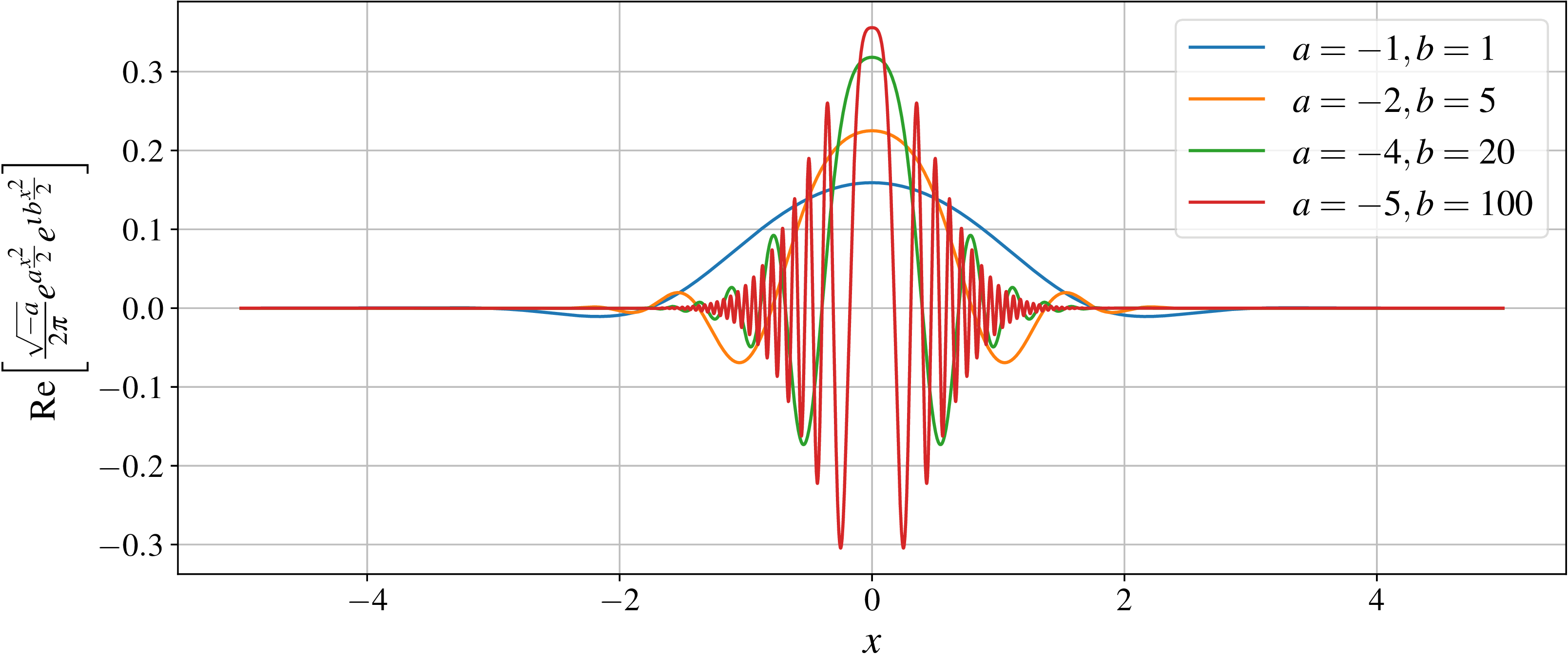
As a last consideration, what would the function $f \in \mathcal{H}$ look like in the case of equality in Eq. \eqref{eq.proof}? For this, we work our way back to the Schwarz inequality applied to Eq. \eqref{eq.interm}, and examine the equality case. We have: \(\begin{align} \left| f^\dagger \hat{X}^\dagger \hat{D}_X f \right| = \left|\hat{X} f\right| \left|\hat{D}_X f\right| \label{eq.schwarzequality} \end{align}\) … which conteptually means that the Hilbert space “vectors” $\hat{X}f$ and $\hat{D}_X f$ are in the same direction and are therefore related by a constant scalar multiple $C_0 \in \mathbb{C}$: \(\begin{align} \hat{D}_X f &= C_0 \hat{X} f \\ \Longrightarrow \frac{df}{dx} &= C_0 xf \\ \therefore \frac{df}{f} &= C_0 x~dx \label{eq.folde} \end{align}\) and we are reduced to solving a good old first-order ordinary differential equation! With an appropriate boundary condition $f(x_0) = f_0$, we get: \(\begin{align} \ln\frac{f}{f_0} &= \frac{C_0}{2} \left(x^2 - x_0^2\right) \\ \therefore f(x) &= \underbrace{\left(f_0 e^{-\frac{C_0 x_0^2}{2}}\right)}_{\equiv A_0 \in \mathbb{C}} e^{\frac{C_0 x^2}{2}} \label{eq.finalsoln} \end{align}\) For the solution in Eq. \eqref{eq.finalsoln} to belong in $\mathcal{H}$ (i.e., to be square-integrable), we require that Re$(C_0) < 0$ (failing which the function diverges). Thus with $C_0 \equiv a + \iota b$ with $a < 0$, the last issue to address in completely specifying $f(x)$ is its normalization. We arbitrarily require that the signal energy $\left|f(x)\right|^2 = 1$ unit, and choose $A_0$ in Eq. \eqref{eq.finalsoln} appropriately. This finally gives us: \(\begin{align} f(x) = \frac{\sqrt{-a}}{2\pi} e^{a\frac{x^2}{2}} e^{\iota b\frac{x^2}{2}} \label{eq.muw} \end{align}\) Such a function, with $a \in \mathbb{R}^-$ and $b \in \mathbb{R}$, will always satisfy $\sigma_x^2 \sigma_k^2 = 1/4$ and is called a minimum uncertainty wavepacket, essentially a Gaussian with a phase factor. The real parts of these functions look like this: