A way to quickly generate spherical meshes recursively from Platonic solids, with a Matlab/Octave implementation.

Introduction

This post describes an algorithm I devised to refine a geodesic Delaunay mesh to the desired resolution. It was motivated by an unrelated problem in solid state physics (my primary interest in my doctoral research days), but I imagine it can be handy in a large variety of computer graphics applications where mesh refinement is required.

The exercise was motivated by the old trick of starting out with a suitable Platonic solid (specifically, a regular tetrahedron, octahedron or icosahedron), recursively bisecting its edges and then projecting the points back on to a sphere. These Platonic solids in particular have exclusively triangular faces. Since at each bisection step a triangle results in four “children” triangles, this method essentially grows a quadtree of mesh elements. The higher the “generation” of this recursion, the finer the mesh obtained on the sphere, with a generation of $0$ resulting in the Platonic solid itself (see figure below).

This method is well-known to people who need to do complex simulations on a spherical surface, such as in earth and planetary sciences. You can read a sophisticated analysis of the mesh generation method here. Being a recovering Matlab addict who has grown to be anal retentive in coding practices, I wondered what would be the most efficient way to generate the list of nodes and faces in Matlab with this quadtree approach, without actually building the quadtree. This resulted in an implementation that I’ve since uploaded onto FileExchange. I’m personally quite proud it because I think it makes great use of the pre-compiled routines and phenomenal vectorization capabilities that Matlab has to offer, while elegantly keeping track of the new mesh vertices and faces that are created at each recursion. Here is a runtime benchmark of $100$ trials of the icosahedral mesh from generations $0$ through $7$ i.e. the mean runtime for the line of code:

[ P, tri ] = generateSphereMesh( gen, 'ico' );

where gen ranges from 0 to 7.

This was run on Octave 4.2.2 on an old Thinkpad T410i laptop with its Intel Core i3 running Ubuntu 18.04. This highly efficient runtime, however, appears to have happened to the expense of readability. This post is intended as a simple tutorial in this bisection-without-a-quadtree approach to generating spherical surface meshes, as well an explanation of my own implementation. In the process I’ll touch upon a few little geometric and book-keeping tricks that I use whenever I have to code in Matlab or Octave, and which I hope you find useful as well!

The bare-bones pseudocode to go from Platonic solid to full geodesic mesh is:

Get mesh for Platonic solid (these nodes already live on a sphere)
n = 0;
for n <= generation:
	Bisect each triangle edge to create 4 children triangles
	Project each new bisector node back on to the sphere
	n++
endfor

It turns out that this can be implemented in Matlab with only one for-loop, the one you see in the pseudocode above. The bisection and projection steps do not in fact require a for-loop over the set of triangles or nodes, as I’ll demonstrate soon enough.

Mesh representation

I’ve adopted a fairly simple convention to represent Delaunay surface meshes in 3D, namely using two arrays:

A $3 \times M$ array of doubles (denoted “P” in code), representing $M$ points in 3D space.
A $N \times 3$ array of ints (denoted “tri”), each row representing the column indices in P that stand for the vertices of the triangular mesh element. The numbers in tri range from $1$ to $M$, in keeping with the $1$-indexing convention of Matlab/Octave.

As an example, shown below is a 2-element mesh (black) that has undergone a single refinement step through edge bisection to give a refined mesh (red) of 9 nodes (4 old, 5 new) and 8 elements (triangles).

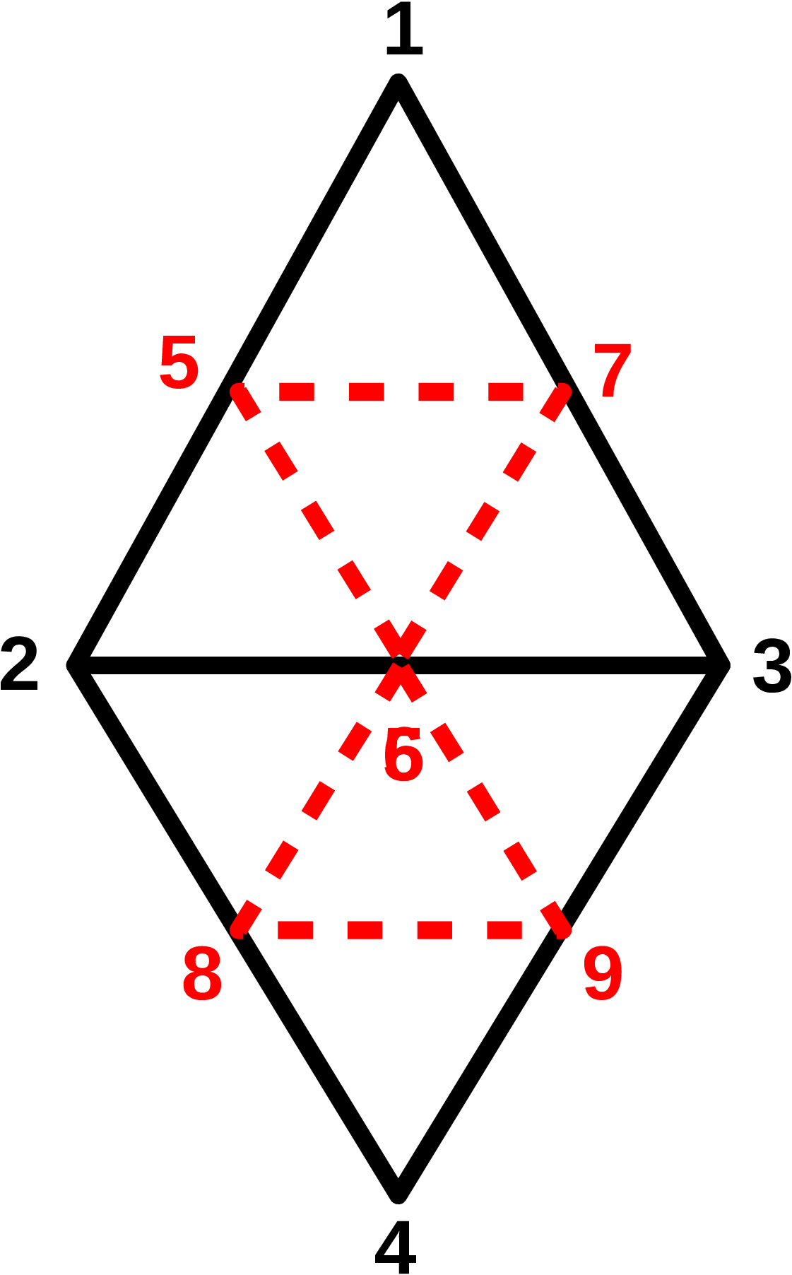The array P in the original mesh would be of size $3 \times 4$ with each column a unit vector, and tri would be (in Matlab notation):

tri = [ ...
	1 2 3 ; ...
	3 2 4   ...
];

The problem statement is to design a refinement step to obtain a new array Pnew of size $3 \times 9$ (each column a unit vector) and a mesh array triNew which is:

triNew = [ ...
5 7 ; ...
2 6 ; ...
5 6 ; ...
6 3 ; ...
2 8 ; ...
8 9 ; ...
9 3 ; ...
8 4   ...
];

…the idea being that this refinement step can be repeated for the desired number of “generations” in the pseudocode above. To most programmers, this problem immediately suggests a recursive solution, which many including myself may find “elegant enough” (to iterate is human, to recurse, divine, remember?). There is, however, extra book-keeping work to be done to take care that nodes are not multiply labeled and preserving the winding order (right- or left-handedness) of each mesh element. By this last point I mean that in triNew, the rows [1 5 7 ] and [ 5 7 1 ] are equivalent and correspond to the same surface normal in the sense of a geometric curl, but are not equivalent to [5 1 7 ]. The issue of handedness of a mesh element is important in many sophisticated meshing libraries, DREAM.3D being the one from work that I’m most familiar with. The point of this post is to describe an even more elegant way to do the refinement step while addressing these and other book-keeping issues.

To achieve a single refinement step on the mesh defined by P and tri, we first need to determine the unique triangle edges from tri. This is done simply by:

edges = [ tri(:,[1 2]) ; tri(:,[2 3]), tri(:,[3 1]) ];
edges_sorted = [ min( edges, [], 2 ) max( edges, [], 2 ) ];
edges_unique = unique( edges_sorted, 'rows' );

It is now possible to bisect all the edges in one go by simply doing:

Pnew = 0.5 * ( P(:,edges_unique(:,1)) + P(:,edges_unique(:,2)) );
Pnew = Pnew ./ repmat( sqrt( sum( Pnew.^2 ) ), 3, 1 );

The last line is a tight, vectorized alternative to the following boring but readable code:

for n = 1:size( Pnew, 2 )
	Pnew(:,n) = Pnew(:,n) / norm( Pnew(:,n) );
end

We now have in Pnew the unique list of edge bisectors, projected back on to the sphere (points 5 through 9 in the figure above). The new node list is simply:

P_refined = [ P Pnew ];

with the understanding that if the original P contained $M$ points, then the nodes in Pnew are indexed from $M+1$ onwards.

Much trickier is how to get the new mesh connectivity triNew. It is here that I need to give a shout out to my favorite among Matlab core routines, ismember. The sheer versatility and flexibility of this function is the reason I was able to solve thousands of little algorithmic issues in the past. The absolutely neatest, cleanest and best way in my opinion to assign indexes to the new nodes determined earlier is like this:

[ ~, idx ] = ismember( edges_sorted, edges_unique, 'rows' );
idx = idx + M; 			% this does the M+1 offset in one shot

This comes from recognizing that there are as many new nodes as there are triangle edges, since each new node is associated with the bisector of an edge. Once this is done, it is a trivial matter to collect triplets of node indexes to form triNew. See how this is done for one refinement step in the refineMesh function.

So that’s about it. Do let me know on the Mathworks page if you find this code useful, or if you have any other questions!